Testing impedance of broadside-coupled differential pairs without ground

Application Note AP8154

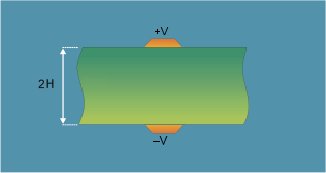
This note, provided for historical information only, refers only to legacy equipment and methods and has been superseded by AP153

Background

This note considers modelling and testing broadside-coupled pairs without grounds.

Consider the structure pictured below – this is a broadside-coupled differential structure.

From a modelling standpoint the structure is like a paired wire transmission line. However the questions arise – how do you model the structure with the Si8000/9000 field solvers and as this is a differential structure but with no ground plane how should you test the impedance?

Fig. 1 Broadside-coupled differential structure

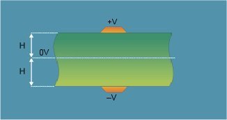
When the tracks are driven in equal but opposite sense the potential at every point equidistant from the two is always 0V (half way between +V and –V). We can use this to our advantage because those points form a virtual ground plane which lies exactly equidistant from each track.

Here's the same structure as in Figure 1 above but showing this virtual ground plane – Figure 2, right.

Fig. 2 Broadside-coupled differential structure

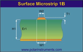
Modelling this structure

The Si8/9000 field solvers do not include a structure exactly like this, but do offer the Surface Microstrip structure – shown in the figure below – which is exactly half of it.

The track in Figure 3 corresponds to the upper track in Figure 2, and the planes correspond. By turning Figure 3 upside down, the track corresponds to the lower track in Figure 2.

Notice the significance of H in the three figures, where H1 in Figure 3 = H in Figure 2.

Fig. 3 Surface Microstrip

The impedance of the differential pair shown in Figure 1 will be the same as their impedance in Figure 2, which in turn will be twice the impedance of the Surface Microstrip in Figure 3. This is because in the structures shown in Figure 1 and Figure 2 both signal tracks are driven, one by +V and the other by –V, so the total driving voltage = +V – (–V) = 2V which is double that in Figure 3. However, the resulting current will be the same and therefore the impedance is double.

So, in order to calculate the differential impedance of Figure 1, simply calculate the impedance of Figure 3 and double it. The Si8000/9000 Quick Solvers are convenient to use for this purpose.

When choosing a suitable model for differential structures look for virtual ground planes between differential tracks to see if a single ended model with ground can be adapted to fit your needs. The virtual ground is a useful tool – and at first sight it may not be obvious that one exists between two conductors driven differentially. Look beyond the obvious to see if this tool can be adapted to suit your needs and use it to your advantage.

Testing the structure

In the structure to be tested all the signal current flows out through one conductor and the return current comes back through the other. As noted earlier, with a signal of equal positive and negative going potential a virtual ground exists midway between the two traces.

How do I connect probes to this?

Imagine using a differential probe with + on one line and – on the other – you are left with nowhere to connect the ground. So in order to test you need to think of this structure as a single ended transmission line and consider connecting to it via a single ended probe. The signal goes to one side of the transmission line and the ground connects to the other.

Using a single ended TDR and probe connection you can connect the probe either way around and measure the impedance of the structure using the system set for single ended measurements. The measurement returned will represent the differential impedance of the transmission line. For this structure this will equal Zo, the single-ended impedance.

Footnote by Dr Alan Staniforth

The impedance of the structure is the ratio of the voltage between, and the current in, the conductors. The concept of driving the conductors as a differential pair implies the presence of a zero voltage ground. The definition of the controlled impedance for this configuration does not require a ground. Hence, without loss of generality, one conductor can have zero voltage assigned to it.

Thus only a single-ended measurement is required, even though one pin of the measurement probe is at ground potential. A three pin differential measurement probe requires a track configuration which already has a ground to which the ground pin is connected. A differential probe, in practice, measures the impedance between the two active pins and the ground pin. The differential impedance is calculated from these two impedances. If the ground pin is not connected, the impedance at the active pins will be incorrect and so will be the differential impedance.