|
|
|
|
|
|
Using the Si9000e sensitivity analysis to graph multiple impedances
Application Note AP8188
|
|
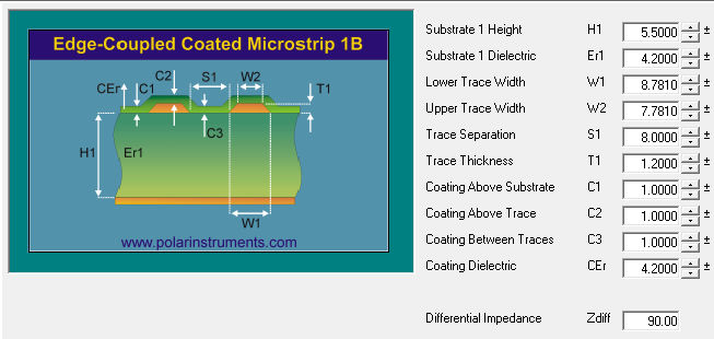
Note: this application note refers to the Polar Si9000e Transmission Line Field Solver only One of the more popular modelling questions that we are asked is, "How do I use the Polar Si9000e field solver to achieve both a differential (Zdiff) and common mode (Zcommon) requirement?" For example, USB 2.0 guidelines specify routing the DP/DM signals with 90 ohms differential impedance, and 22.5~30 ohms common impedance. This note describes how to use the Si9000e's sensitivity analysis to achieve both the differential (Zdiff) and common (Zcommon) specifications. Using Constant Impedance vs Changing Parameters mode, setting the Target Impedance to 90 ohms and looking at the Zdiff, Zcommon or All Impedance display series allows the user to select a W1 / W2 / S1 combination that meets both differential and common impedance requirements. In the Si9000e, click the Lossless Calculation tab. Select the Edge-Coupled Coated Microstrip 1B structure; use the default structure parameters but change the substrate height, H1, to 5.5 mils and calculate the impedance; set a target differential impedance, Zdiff, of 90 ohms and goal seek on trace width to achieve 90 ohms. Parameters are shown below.
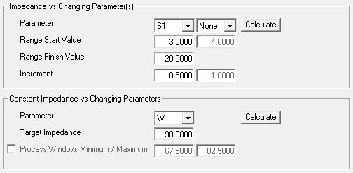
Using the Si9000e sensitivity analysis Switch to the Si9000e Sensitivity Analysis tab. Under the Impedance vs Changing Parameter section set the Parameter to trace separation, S1, set the Range Start Value to 3 mils and the Range Finish Value to 20 mils – choose an increment of 0.5 mils. In the Constant Impedance vs Changing Parameters set the Parameter to trace width, W1 and the Target Impedance to 90 ohms. Click Calculate in the Constant Impedance vs Changing Parameters section.
The Si9000e Constant Impedance plot charts trace width v trace separation over the selected range of values of S1 while maintaining a constant value of 90 ohms differential impedance.
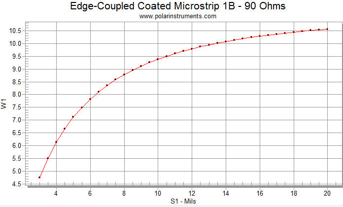
A subset of the Si9000e's sensitivity analysis results as trace width and separation vary is shown below.
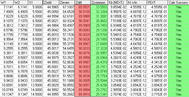
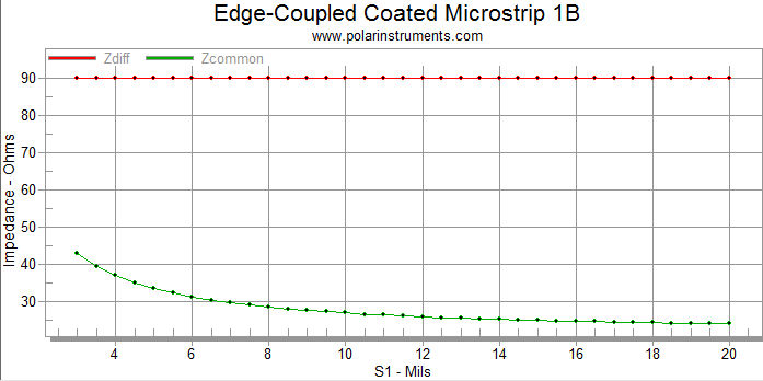
The Si9000e Results tab shows W1 / W2 / S1 changing; the differential impedance, ZDiff, calculates to 90 ohms but you can also see how the common impedance value, Zcommon,changes for each W1 / W2 / S1 combination of parameter values. This data can be exported to other tools (for example, Microsoft Excel®) for further analysis. The associated graph (showing Zdiff at 90 ohms and Zcommon varying between 44 ohms and 24 ohms) is shown below.
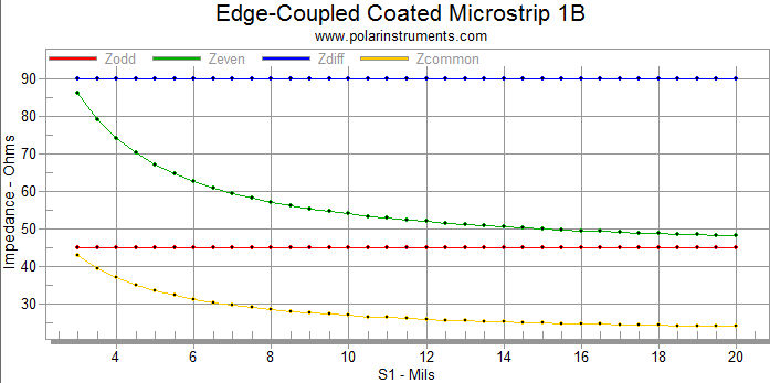
Displaying all impedances The Si9000e sensitivity analysis includes graphing for differential, common, odd and even mode impedances along with near and far-end crosstalk. Change the Display Series from Zdiff, Zcommon to All Impedances. The Si9000e plot below shows differential, odd mode, even mode and common impedances as S1 increases and W1 changes while maintaining the target differential impedance of 90 ohms.
|