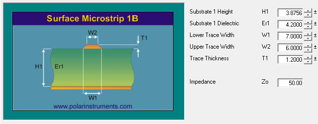
How does TDR risetime affect the measurement of impedance?

The Polar CITS880s TDR is specifically designed to measure controlled impedance test coupons and test traces and is an excellent choice for many impedance measurement applications. It combines measurement speed for high throughput, ease of use and protection against ESD damage to make it especially suitable for a manufacturing test environment.

Many people assume that as the speed of their signals increase, they need to measure impedance with a “higher speed” TDR. The "higher speed" specification in question is the rise time of the pulse generated by the TDR. As it turns out, you will measure the same impedance on a PCB test coupon regardless of the TDR rise time.

As a matter of fact, if you do use a “laboratory class” TDR with a fast rise time it is usually recommended that you invoke the “filter” function on the TDR to slow the rise time down to reduce ringing and noise. This allows you to make a more accurate impedance measurement on the flat part of the waveform. Please see Polar Application Note AP168 The effect of risetime on TDR measurement of impedance.

In the CITS880s impedance is measured against time or distance and is displayed on the vertical axis. The primary reason to use a TDR with a faster rise time is for better resolution of time and/or distance measurements. If you are characterizing a connector, or other very short type of interconnect, then a faster rise time will allow you to see anomalies that would be missed with a slower rise time. However, PCB test coupons are generally six inches long (see IPC standard IPC-2141A Design Guide for High-Speed Controlled Impedance Circuit Boards) so the faster rise time buys you nothing – except increased susceptibility to ESD damage.

Change of impedance with frequency

Impedance, of course, changes with frequency. However, many customers are very surprised to learn that the changes actually occur at “relatively” low speeds, and then flatten out. If you use Polar's Si9000 frequency dependent field solver to model a PCB trace and plot the impedance magnitude, you can observe the effect.

The Si9000 includes both lossless and frequency dependent calculations. In the illustration below, using lossless modelling, the Si9000 calculates the parameters of the surface microstrip structure for 50 Ohms.

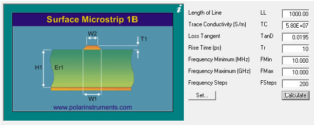
The Si9000 is then switched to “frequency dependent” modelling and calculates the loss, skin depth, s-parameters, etc. for the structure. The same structure is shown below, followed by the associated impedance magnitude graph:

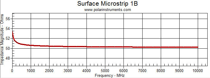
In this case the impedance is charted over a frequency range from 10 MHz to 10 GHz and you can see that the impedance magnitude has settled out well under 1 GHz.

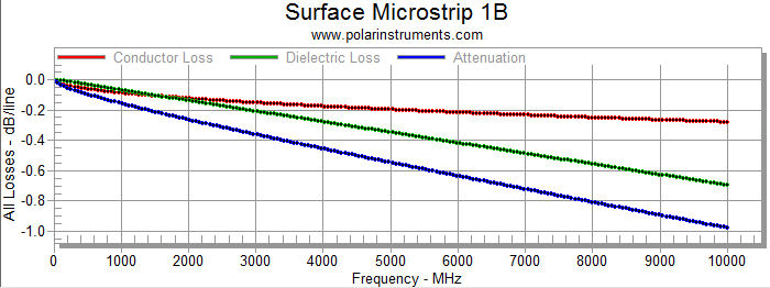
Loss v frequency

Loss, of course, changes significantly with frequency and clearly becomes a much bigger problem as the frequency increases. Using the same structure as above, the Si9000 charts the losses you can expect to see along the trace – the red trace (Conductor Loss) the copper, the green trace (Dielectric Loss) charts loss due to heating in the dielectric and the blue trace (Attenuation) displays the total insertion loss.

Modeling and measuring loss

The modelled trace is one inch long, so the vertical axis units of “dB/line” is also “dB/inch”, which can be scaled for longer traces by simple multiplication. In addition to the Si9000e Insertion Loss GHz Transmission Line Field Solver, Polar also produces the Atlas Si Insertion Loss Test System for measuring loss. If your frequency of interest is much above 2-4 GHz then you should also consider measuring insertion loss. Please contact Polar if you would like further information about either software package.